
A Chess Puzzle, Part VII Episode 2 : The Rational Super Queen
Part VII Episode 2 of A Mathematical Chess Puzzle:
- Part I: The Infinite Chess Board
- Part II: Ruminations
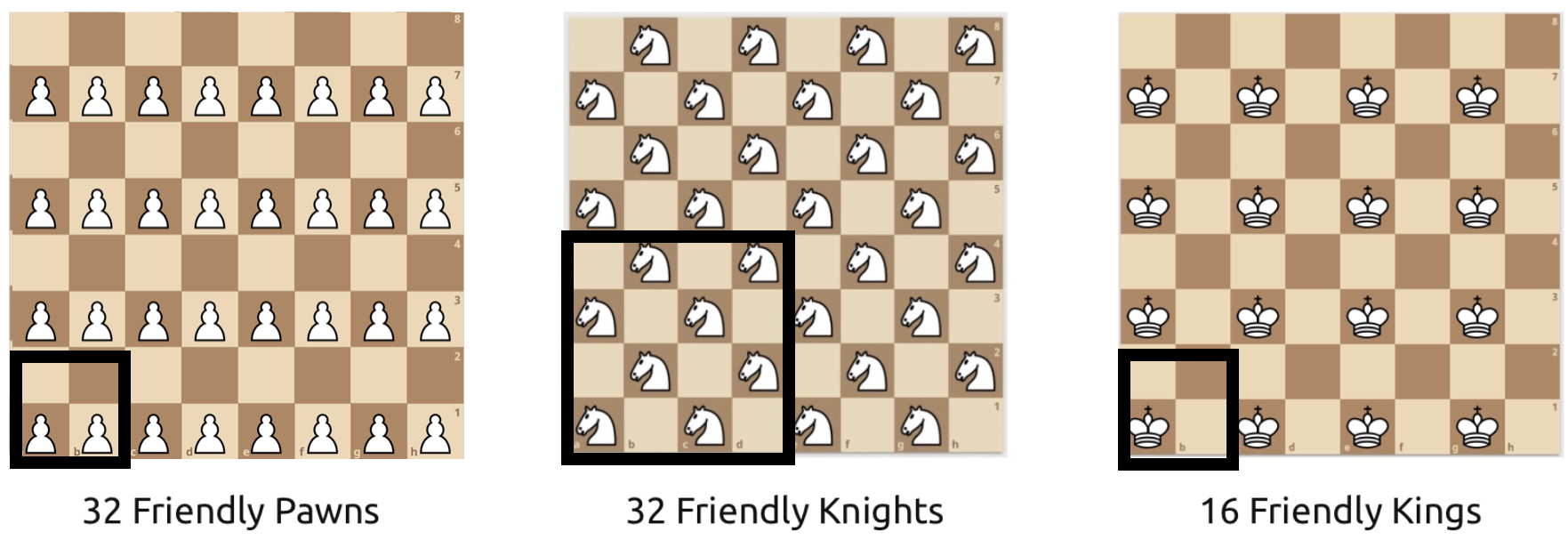
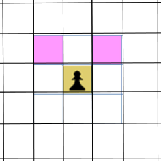
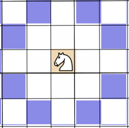
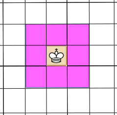
- Part III: The Pawns, Knights and Kings
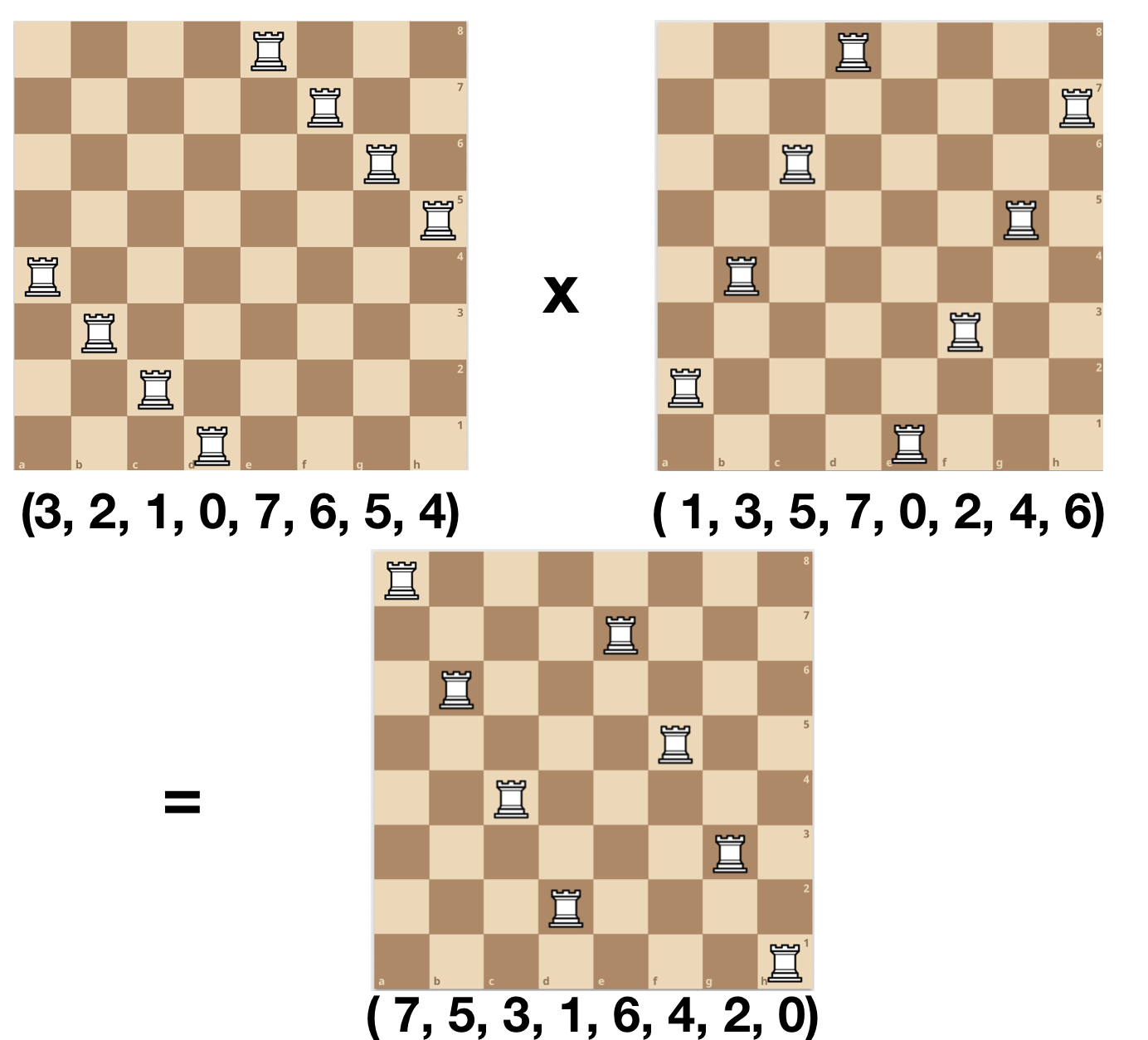
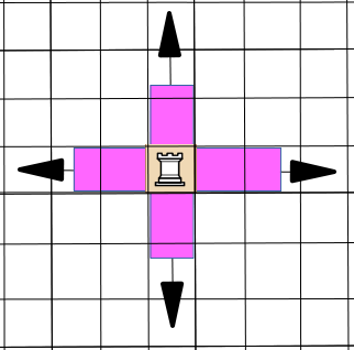
- Part IV: A Group of Rooks
- Part V: Rooks and Topology
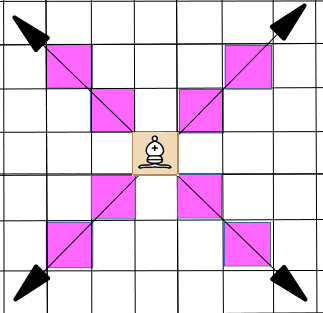
- Part VI: The Bishop
- Part VII Episode 1: The Fractal Queen
- Part VII Episode 2: The Rational Super Queen
- Part VIII Conclusion: The Transfinite Super Queen and Beyond
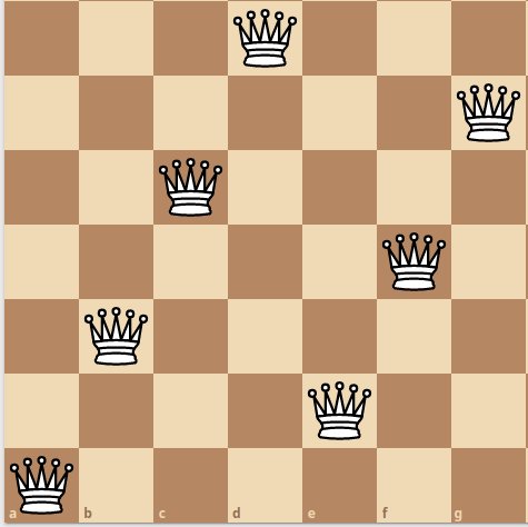
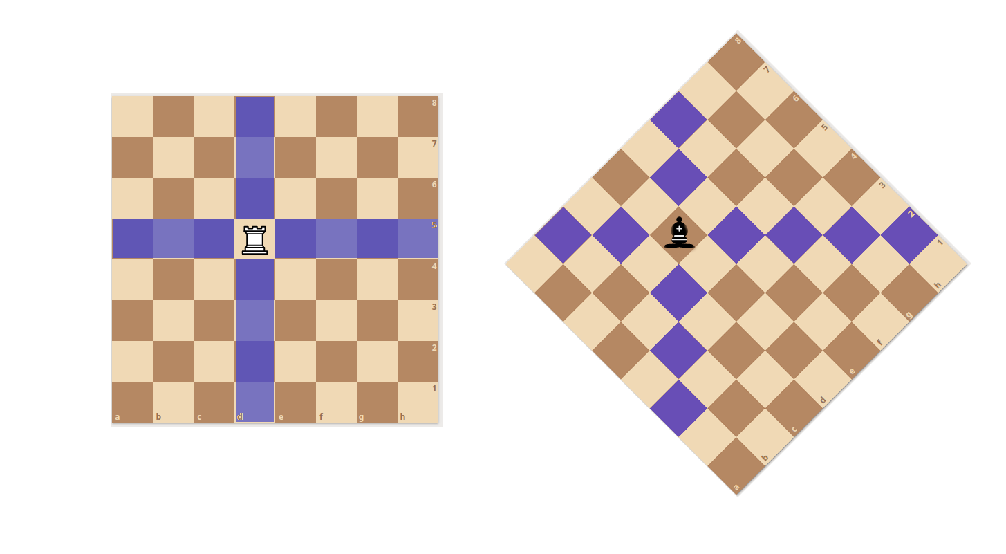
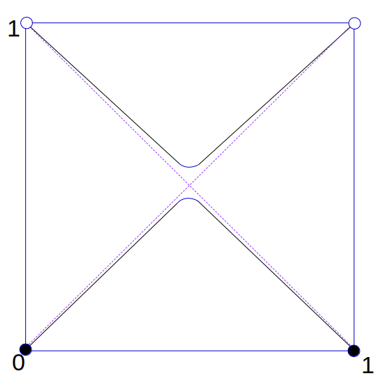
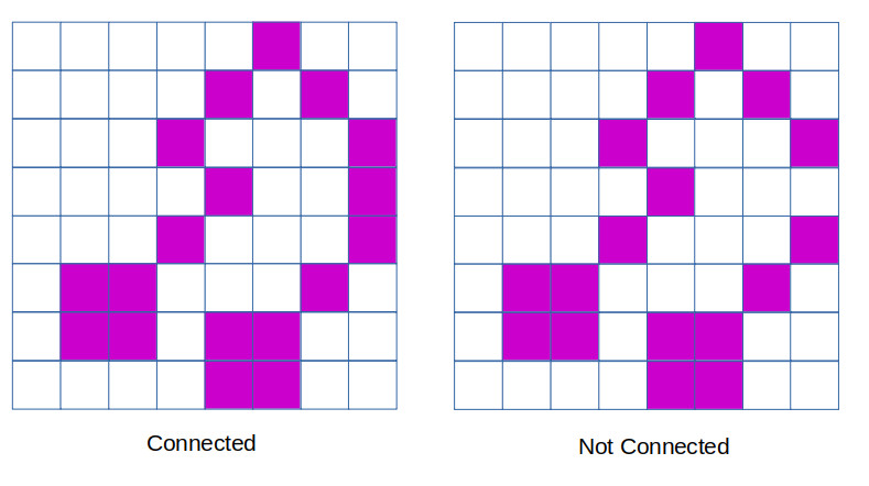
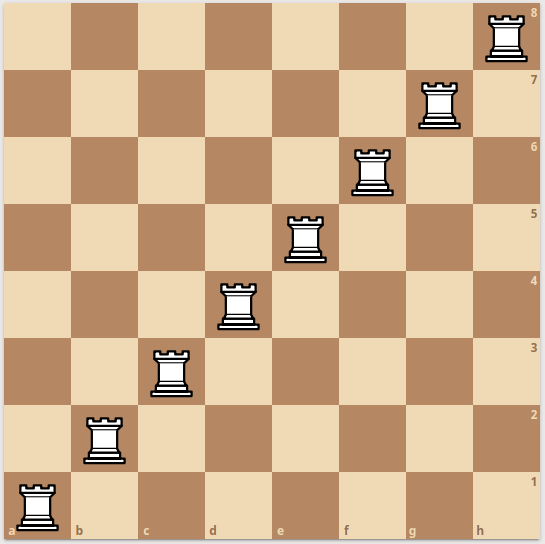
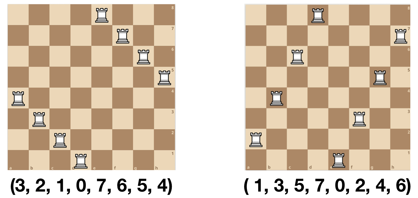
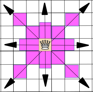
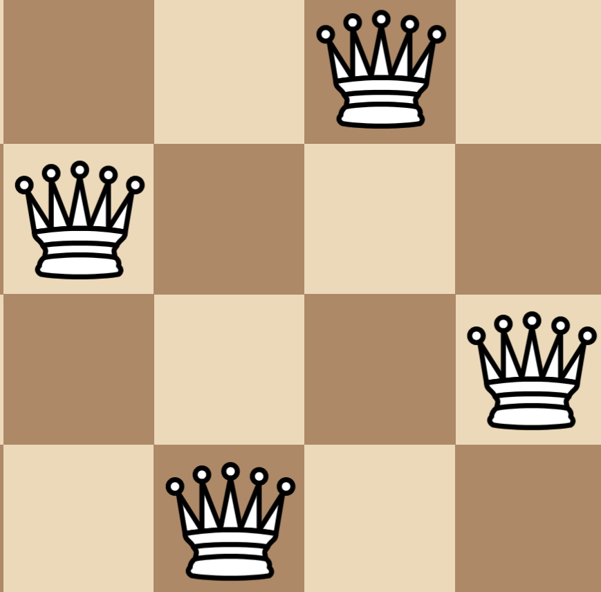
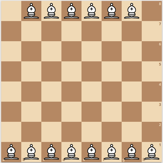
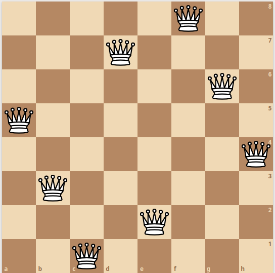
We are nearing the end, but still there is the tallest mountain to climb. We need to prove the SUPER QUEEN THEOREM, which says that not only is there a chess position $Q$ to the unguarded queen problem on the unit continuum board $B_c$ (where $c$ are is understood as all reals in the open unit interval (0,1)), but that in fact that solution satisfies the Super Queen property — which is to say, that not only is there exactly one queen on every rank and file (“Rook Maximal”), but that there is also exactly one queen on every diagonal (“Bishop maximal”). This is not possible on finite boards because we run out of places on diagonals to put the queens that don’t attack an existing queen by a rook move.
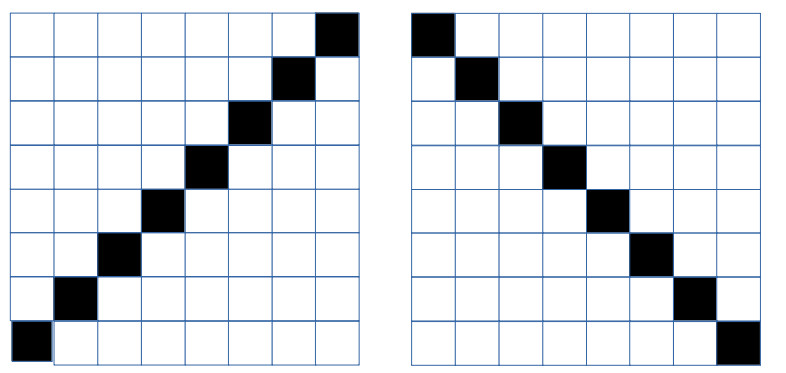
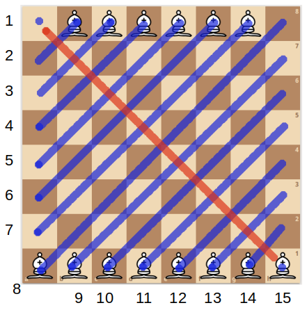
Note: we exclude the endpoints 0 and 1 from the intervals to remove the “degenerate” diagonals on the corners, and so ensure that all rows, columns and diagonals are of positive linear measure. If they were included, then only one of the two degenerate diagonals through (0,0) and (1,1) respectively could be admitted and the “super queen” property would not hold.
Climbing an Infinite Ladder
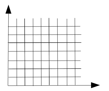
To prove this theorem, as mentioned in the previous post, we will need to use a technique called Transfinite Induction. This is a concept which extends a more conventional technique called Mathematical Induction. The general idea of regular induction in mathematics can be expressed using the metaphor of a ladder:
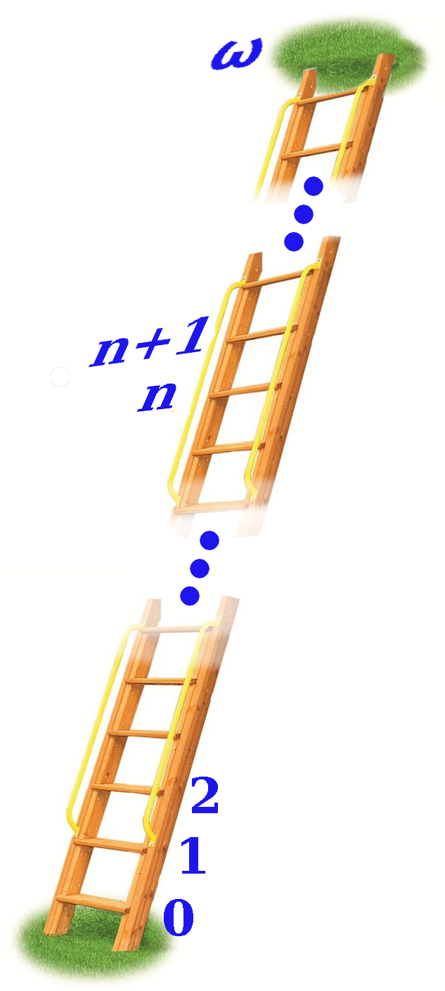
Infinite Ladder
Mathematical Induction: If you can prove that
- you can get on the first rung of a ladder, and
- you can also prove for any N that
if you can get to rung $N$,
then you can also get to the next rung $N+1$,
then you have proven you can go all the way up the ladder.
This does not seem very deep, and in fact seems obvious, but it is a technique used in many parts of mathematics. For example, consider the theorem:
THEOREM: For every integer $n \ge 1$, the odd sum $1 + 3 + 5 … (2n-1)$ is a square, and in fact
$$S_n = 1 + 3 + 5 … (2n-1) = n^2\tag{**}$$
For example, for $n=1$, $1 = 1^2$, for $n=2$, $1 + 3 = 4 = 2^2$, and so on.
PROOF: We shall use (regular) mathematical induction. The first step is to prove we can get on the “first rung”, so we look at $n=1$ and can see that indeed $1 = 1^2 = (2n-1)^2$. For the next step, suppose that formula (**) holds for a specific $n = N$, that is, for a specific $N$ we have:
$$S_N = 1 + 3 + 5 … (2N-1) = N^2\tag{***}$$
We need to show that (**) also holds for $n= N+1$. We can write
$$S_{N+1} = 1 + 3 + 5 … (2(N+1)-1)^2$$
$$ = 1 + 3 + 5 … + (2N -1)^2 + (2(N+1)-1)^2$$
which by definition can be rewritten:
$$ = S_N + (2(N+1)-1)^2$$
and by the assumption (***) we have
$$ = N^2 + (2(N+1)-1)^2$$
which simplifies to
$$ = N^2 + 2N + 1 = (N+1)^2$$
which is formula (**) with $N+1$ substituted for $n$. We have just proved the second part of induction, which is that if (**) is true for $N$ then it is also true for $N+1$, and so the theorem is proved. QED.
The Rational Super Queen
As a first step toward proving the Super Queen Theorem on the transfinite board $B_c$, we will first prove the analogous theorem on the rational unit board $B_{\mathbb{Q}}$, where $\mathbb{Q}$ is understood as the set of all rational numbers between 0 and 1 exclusive.
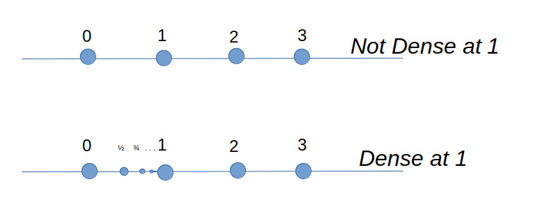
Referring back to the previous article on the Rook, both the rational unit board and the omega board have a countable infinity of “squares”. And as in that case, what makes the situations different is that the omega board (whose coordinates are integers) has a discrete topology, while the rational numbers are dense, and no square has a unique square “next to” it.
It should be noted that when restricted to just rational points, the concept of rook and bishop lines restricted to $B_{\mathbb{Q}}$ makes sense. The reason is that for any two “rational” points $p,q \in B_{\mathbb{Q}}$,, and any two rook or bishop attack lines $\lambda_p,\lambda_q$ which pass through $p$ and $q$ respectively, that their intersection is either empty or another rational point $r \in B_{\mathbb{Q}}$. That is, you will never have two points on the board whose common points of attack are irrational points outside of $B_{\mathbb{Q}}$. (Proof left to the reader)
Let us define $\Lambda$ to be the set of all rook and bishops lines (ie, all Queen lines) in $B_{\mathbb{Q}}$. Then we have
The Rational Super Queen Theorem: There exists a queen position $Q$ on the rational unit board $B_{\mathbb{Q}}$, such that for every queen line $\lambda \in \Lambda$ the intersection $\lambda \cap Q$ has exactly one point $q \in B_{\mathbb{Q}}$. That is, every Queen attack line in $B_{\mathbb{Q}}$ is occupied by exactly one queen in the position $Q$.
We will prove this theorem by (regular) mathematical induction. To do this we will need some definitions and to prove some lemmas first.
Definition: a set $S$ is Well Ordered if there is an operator (which we will call $\le$), such that for all $x,y,z \in S$ we have
- $x \le x$
- Either $x \le y$ or $y \le x$
- if $x \le y$ and $y \le z$ then $x \le z$
- if $x \le y$ and $y \le x$ then $x = y$
- (Well Ordering): For any subset $T \subset S$, there exists a “smallest” element $x \in T$, ie, so that $x \le y$ for all $y \in T$.
The first four conditions describe “total ordering”, while the fifth (important) condition is what makes a “well ordering”. The principle of Mathematical induction is equivalent to the statement that the natural numbers $\mathbb{N}$ is well ordered.
Example 1: The positive integers $\mathbb{N}$ are well-ordered with the usual numeric ordering $\le$.
Example 2: The set of all integers $\mathbb{Z}$ is NOT well-ordered under $\le$, because $\mathbb{Z}$ itself is a set having no smallest value (violating condition 5).
Theorem 1: The rational points $(x,y) \in B_{\mathbb{Q}}$ have a well ordering (but not the usual one $\le$).
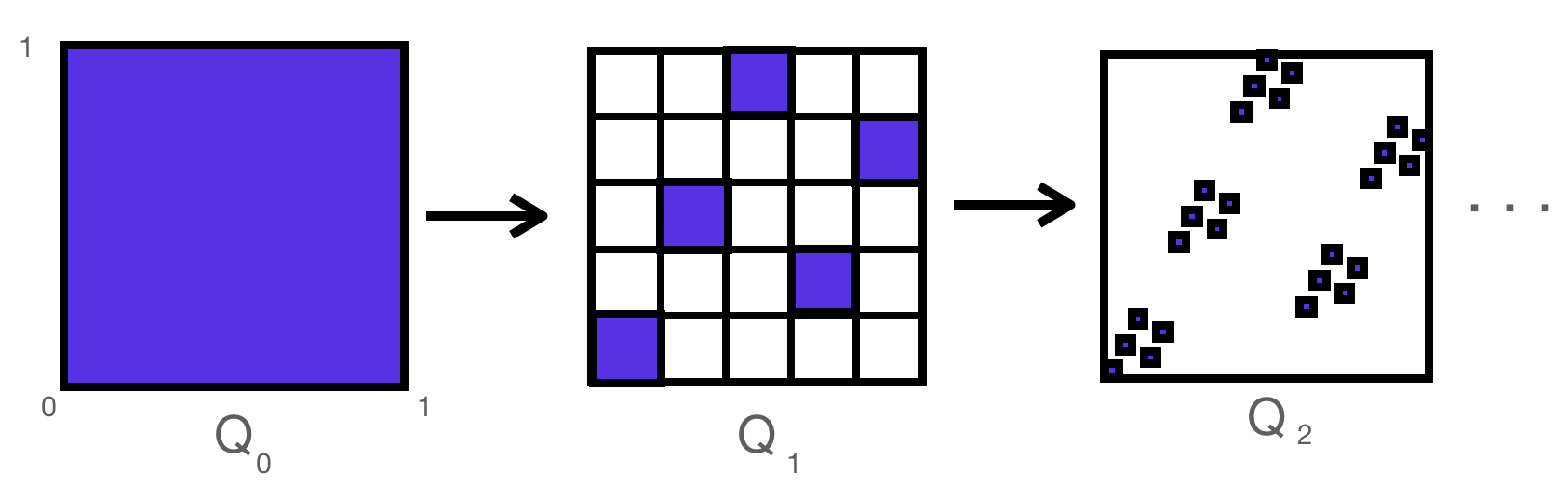
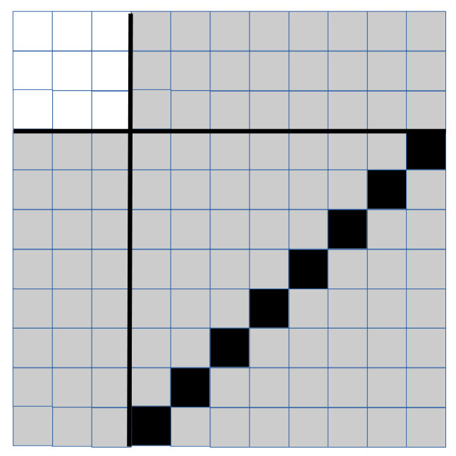
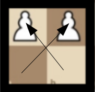
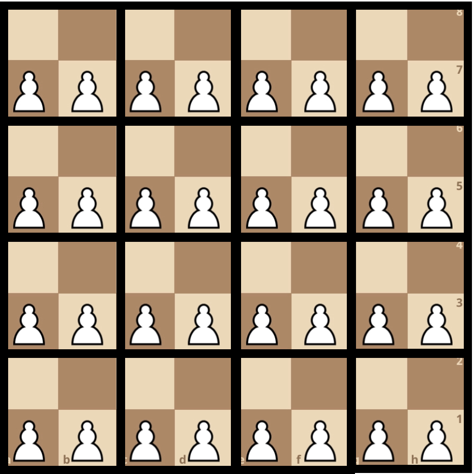
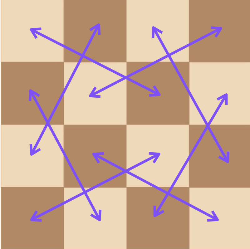
Proof: It is known that the positive rational numbers $\mathbb{Q}$ are countable; that is, that there exists a function mapping the natural numbers $\{1,2,3,…\}$ to $\mathbb{Q}$ in a 1-to-1 way. To see that, observe that they can all be represented as fractions $p/q$ in a square array whose x and y coordinates indicate the numerator and denominator (below). Note that fractions that are not in simplest terms (e.g. 2/2) are skipped.
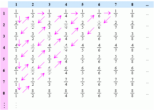 As the arrows suggest, we can then “thread” the numbers onto a line, and number them by the order they appear, like this:
$$x_n = \frac{1}{1}, \frac{2}{1}, \frac{1}{2}, \frac{1}{3}, \frac{3}{1}, . . . $$
$$n = 1, 2, 3, 4, 5, . . . $$
This gives us a function $Q(n)$ which takes the integer $n$ to $x_n$. And so, we can define our new “ordering” (call it $\prec$) on the positive rationals by defining $x_n \prec x_m$ if and only if $n \le m$ in the usual sense. And this ordering is well-ordered, because for any subset $S$ of positive rationals, one simply considers the inverse set $S’ = Q^{-1}(S)$. SInce $S’$ is a subset of the positive integers, there must be a smallest one $m \in S’$, and by definition this is also the “smallest” in $S$, ordered by $\prec$. QED
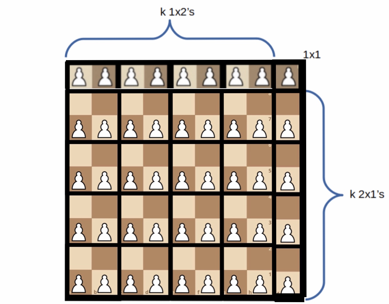
Theorem 3: The rational points $(x,y) \in B_{\mathbb{Q}}$ have a well ordering.
Proof: We can follow a proof that parallels the one just given for Theorem 2. For we can use the inverse function $Q^{-1}(x)$ to map all rational points $(x,y)$ to non-negative integer points $(m,n)$, and by arranging them in a similar grid as above, “thread” the integer grid with a single integer line, and then use the inverse of this mapping to map the well-ordered integers to the rational points. QED
Theorem 4: The set $\Lambda$ of queen lines on the rational board is countable and can be well ordered.
Proof: Each (non-degenerate) queen line can be identified by a pair of distinct rational points $(x,y)$ and $(z,w)$ on the board which belong to it. The rational points are well ordered and (by the same arguments above), the pairs of such points also have a well-ordering.
Proof of The Rational Super Queen Theorem
Our goal is to prove that we can construct a position $Q = \{ q_0, q_1, . . . \}$ on the unit rational board, such that every queen line $\lambda \in \Lambda$ contains exactly one and only one element $q \in Q$.
By Theorem 4, the queen lines $\Lambda$ are countable. This means that we can assign an index $n$ to each of them which might as well be the integers 0,1,2…), which also gives them a well-ordering.
In addition, the points on the rational board itself is countable and has a well-ordering.
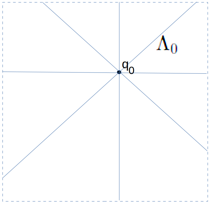
First Step, definining Λ₀
To prove the existence of a position $Q$ we shall use (regular) mathematical induction.
For step zero, we simply define $q_0 = b_0$ where $b_0$ is the first element in the well-ordering of the board. We also define $\Lambda_0$ to be the set of (four) queen lines which pass through $q_0$. Let us also define the set $Q_0 = \{ q_0 \}$.
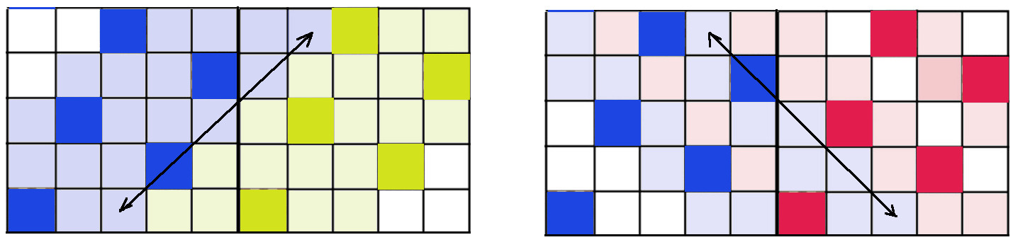
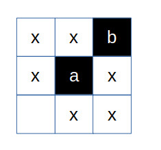
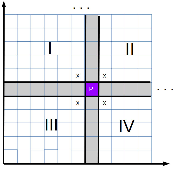
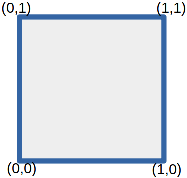
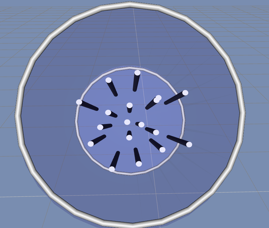
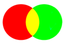
For step 1, we consider the set of all queen lines which are not in $\Lambda_0$, and take the queen line $\lambda = \lambda_\alpha$ whose index $\alpha$ is the smallest among those. We then exclude from this $\lambda$ (considered as a set of points in the board) all points where it 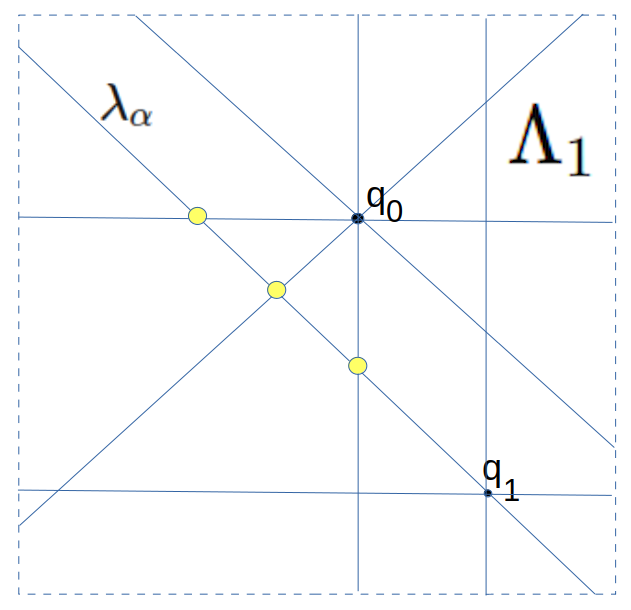 intersects $\Lambda_0$ (shown here in yellow). This intersection is a finite set of points, and so we can pick for $q_1$ any other point on $\lambda$ not in this intersection. We then can define $\Lambda_1$ to be the set of all queen lines which pass through the set $Q_1 = \{ q_0, q_1 \}$. Note that $\Lambda_1 \supset \Lambda_0$ and is itself finite. We also note that any place where $\Lambda_0$ and $\Lambda_1$ share a point, those points are not in $Q_1$.
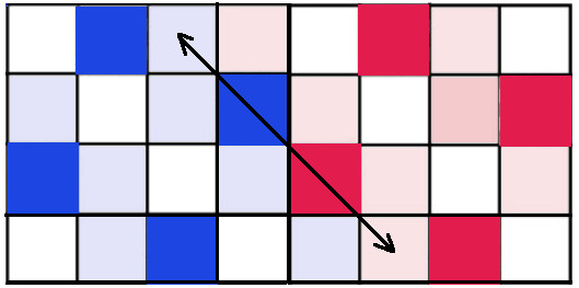
To generalize this last step inductively, for step $n+1$, we consider the set $S \subset \Lambda $ of all queen lines which are not in ${\Lambda_n}$, and among them choose a queen line $\lambda = \lambda_\alpha$ whose index $\alpha$ is the smallest within $S$. We can do this because ${\Lambda_n}$ is a finite set of queen lines, and so the remaining set is non-empty (in fact, countably infinite), and $\Lambda$ is well-ordered. We now consider the set of all intersections of $\lambda$ with lines in ${\Lambda_n}$. As before, this is a finite number of intersections and so we can choose for $q_{n+1}$ any point in the (infinite) queen line $\lambda$ not in this set, and define $\Lambda_{n+1}$ to be all queen lines passing through points $Q_{n+1} = Q_{n} \cup \{q_{n+1}\}$.
We now assert that (1) this tower of inclusive sets
$$\Lambda_0 \subset \Lambda_1 \subset \Lambda_2 . . . $$
is exhaustive, and its union will eventually include every single queen line $\lambda \in \Lambda$. In other words, the union is itself $\Lambda$. And furthermore, (2) the union of the tower of sets
$$Q_0 \subset Q_1 \subset Q_2 . . . $$
is our desired position $Q$ and that every member of $\Lambda$ meets $Q$ in exactly one point. The proof of this is below:
(1) To see that the $\Lambda_n$ tower is exhaustive, assume that this was not the case, and that there was some $\lambda$ that was missing from the tower, and so let us choose $\lambda_\beta$ to be the smallest of these missing ones in the well-ordering of $\Lambda$. But now consider how we constructed the set $\Lambda_{\beta + 1}$. By construction, it was the union of $\Lambda_{\beta}$ with the $\lambda_n$ with the smallest index $n$ which was not in $\Lambda_{\beta}$. But this means that $n$ must be greater than $\beta$, and so $\lambda_\beta$ should have been chosen at that step because it has a smaller index and is not in $\Lambda_{\beta}$.
(2) To see that every member $\lambda$ of $\Lambda$ meets $Q$ in at least one point, simply note that $\lambda$ must belong to $\Lambda_n$ for some smallest $n$ (since the union was exhaustive). But $\Lambda_n$ was defined to be all queen lines passing through $Q_n$, and so $\lambda$ must meet at least one element of $Q_n \subset Q$. But the points already chosen were selected from a set that excluded pairwise intersections of members of $Q_n$, and so $\lambda$ cannot possible meet any more than one element (as pairwise intersections were excluded). Hence $\lambda$ meets $Q_n$ at exactly one point, and by the construction, no later $Q_m$ sets meet $\lambda$ at all.
QED
This proof is remarkable, because nothing like it is possible with the finite boards. The thing which makes this work, is that at each step we are only removing a finite number of points from an infinite board, and so we can always find more in the remaining infinite sets to satisfy our conditions. Unlike the finite case, it did not matter whether any “queen line” was a rook or bishop style line. They were each treated equally in the set $\Lambda$ and the process of eliminating candidate points for the next step never exhausted the pool.
Having now proved the “Super Queen” solutions exists for the rational board, we are ready to pull out the big guns in the next post and deal with the Super Queen solution on the transfinite real board.


